Simulation: simulating uncorrelated and correlated random variables

FYI: This is a text about basic simulation, nothing fancy, but you do have to know some basic math and statistics. Nothing special though… they taught me matrices, means, standard deviations and the normal distribution when I was 16 years old. So this stuff is not rocket science at all. It’s useful for people like me but 4 years younger, still looking for the answer to the question I will describe below. It’s useful for people who like finance but don’t have a strong core yet. It’s also useful for people who just want to refresh some things, or for people who want to use some of this stuff in their work. And of course for people who don’t know what simulation means.

Simulation is easy to understand. You just have to recognize that in this world, some things happen by chance. Once you accept that, you can move on and try to understand the process that generates those chances. Once you find that process, you can use simulation to simulate alternative paths. For example: in real life you might toss a coin and get two times heads and three times tails. But on my computer, I can simulate millions of such coin tosses and see what happens each time. I can simulate alternative paths for the coin toisses and many other random things. This is simulation! Simulation is a huge topic, but I’ll focus here on some things that I encountered and for which I believe that the internet does not yet provide an easy peasy lemon squeezie explanation. You’ll find stuff everywhere, but I’ll try to condense it down to the core here. And I’ll try not to be too technical, since technical readers already have a lot of books to rely on anyway.

A while ago I wanted to simulate companies going into default. It’s likely that companies tend to default at the same time. In other words: defaults are correlated. You can ask yourself similar questions when you’re analyzing stock returns, for example. Stocks tend to move up and down together because their returns are correlated. But you can also simulate your pension plan, or even the temperatures in January. You can simulate the numbers of cars that drive past your house or you can simulate the size of different queues in a supermarket. As one of my PhD supervisors always says: “If you are simulating, you are God”. And it’s true, apart from the fact I can’t seem to simulate a higher balance on my bank account. Maybe I can ask my supervisor about that…? Anyway, if you’re in risk management, you want to be able to simulate all kinds of stuff. Why? Because it allows you to look into the future, within the limits of your model, and see the possible scenarios and their probabilities. Banks may want to simulate all the products in their portfolio (bonds, loans, stocks, derivatives, …) and see what can happen within a given period of time, so that they can adequately prepare themselves for some of the worst case scenarios. This is exactly what they do in real life, and this is exactly what I’m studying in my PhD.

1. Simulating random numbers and uncorrelated random variables

If you’re going to simulate, everything starts with random numbers. Simulating random numbers is very easy. For example, in Excel, the RAND() function will return a random number between 0 and 1, which conveniently corresponds to the definition of a probability. A probability, after all, always lies between 0 and 1. Let me just simulate 10 of those numbers right now:

$\begin{bmatrix}0.6853&0.0153&0.4608&0.5975&0.9186&0.3949&0.7921&0.5599&0.3168&0.4258\end{bmatrix}$

Now, because a probability always lies between 0 and 1, we can use these random numbers to draw random values from ANY well-defined probability distribution. Given such a distribution, you can calculate the probability for some value or range of values. But it also works the other way around: you can input a probability and get a value. This is the idea of simulation. Normally you calculate probabilities for values, but now we calculate values for probabilities. And those probabilities are easy to randomly generate, using e.g. Excel. For example, we can use the random numbers above to draw 10 random values from a normal distribution with mean 100 and standard deviation 15. Just use the =NORMINV() function in Excel. You specify a probability, a mean and a standard deviation, and you get the values that you want:

$\begin{bmatrix} 107&68&99&104&121&96&112&102&93&97\end{bmatrix}$

I rounded these numbers. So what do we have now? Well, we have the IQ’s of a group of 10 people, since IQ is normally distributed with mean 100 and standard deviation 15. Neat, huh? But we can also use those 10 numbers between 0 and 1 to simulate 10 stock returns. Suppose those are normally distributed with mean 5% and standard deviation 15% (yes, stocks are risky!), we get something like this:

$\begin{bmatrix}12.2&-27.4&3.5&8.7&25.9&1.0&17.2&7.3&-2.2&2.2\end{bmatrix}$

You can also use other distributions. For example, I can simulate the number of eyes one can throw when playing dice. I just have to multiply the number between 0 and 1 by 6, and then round up. This gives me:

$\begin{bmatrix}5&1&3&4&6&3&5&4&2&3\end{bmatrix}$

Yes, this is all extremely cool, but also very simple.

2. Simulating correlated random variables (e.g. stock returns)

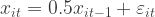
We just simulated some observations for one variable. We can do this for more variables as well. If we copy the approach above for many variables, we get a set of uncorrelated variables. But what about situations in which we want correlation between the variables? For example: what if we want to simulate correlated returns for three stocks? Now before we start simulating, we have to think about how stock prices move. They tend to go up on average, which means they don’t have a constant mean over time. For modeling purposes, this is rather annoying. So the solution is easy: let’s look at returns instead. Let’s say we model them like this:

$R_t = \mu + \varepsilon_t$

This just means that returns at time t, $R_t$ , are always an average $\mu$ plus some random error or “shock” $\varepsilon_t$ . Let’s say we let $\mu$ equal 5% per year and we let $\varepsilon_t$ be a normally distributed independent variable with mean zero and a standard deviation of 15%. Given these assumptions, we can easily simulate say 100 years of $\varepsilon_t$ for each stock and use these to generate the returns for those three stocks. It looks like this:

Of course, this doesn’t look very informative. So let’s take a look at the prices these returns imply, given that all stocks are worth $100 at the start.

These lines look like stock prices. But of course, they are uncorrelated. Simulating correlated random variables is pretty easy, although it may look hard. The first thing you need is a correlation matrix $\textbf{C}$ , for example:

$\textbf{C} = \begin{bmatrix} 1.0 & 0.5 & 0.5 \\ 0.5 & 1.0 & 0.5 \\ 0.5 & 0.5 & 1.0\end{bmatrix}$

This matrix just holds the correlations between each pair of stock returns. Before, we had 100 uncorrelated errors $\varepsilon_t$ for each of the three stocks. In order to transform these to correlated errors, we’re going to put them into a $100\times3$ matrix denoted $\bf U$ . Next, we need to take our correlation matrix $\bf C$ and calculate it’s Cholesky decomposition $\bf L$ , which is a transformation which you can easily calculate using mathematical software. I’m not going to explain in detail what a Cholesky decomposition is, just know that the following applies: uncorrelated variables x Cholesky decomposition = correlated variables. Simply put, a Cholesky decomposition $\bf L$ is a matrix such that $\bf L^{T}L=C$ . Look at the bottom of this post for some VBA code. We get the following:

$\textbf{L} = \begin{bmatrix} 1.0000 & 0.5000 & 0.5000 \\ 0.0000 & 0.8660 & 0.2887 \\ 0.0000 & 0.0000 & 0.8165\end{bmatrix}$

Now we just multiply our matrix of uncorrelated errors $\bf U$ with the Cholesky decomposition $\bf L$ , to get a $100\times3$ matrix of correlated errors $\bf E$

$\bf E=UL$

And indeed, when we use these correlated errors in order to compute returns and prices, we find the following:

Maybe it’s hard to see that the first graph has uncorrelated returns and the second one has correlated returns. But if we calculate the empirical correlation matrices of the uncorrelated and correlated returns, we get respectively:

$\begin{bmatrix} 1.00 & 0.10 & -0.31 \\ 0.10 & 1.00 & -0.01 \\ -0.31 & -0.01 & 1.00 \end{bmatrix}$ and $\begin{bmatrix} 1.00 & 0.52 & 0.39 \\ 0.52 & 1.00 & 0.56 \\ 0.39 & 0.56 & 1.00 \end{bmatrix}$ .

The difference is clear. In the first one, all the correlations are close to 0, while in the second one, all the correlations are close to 0.5 (apart from the elements on the diagonal, which are of course all 1). Of course they are not perfectly equal to 0 or 0.5, but that’s because we’ve only simulated a sample. The correlation matrix $\bf C$ is just the one that holds in the population, but in finite samples the correlation matrix will obviously differ from sample to sample. For example, you can see that even if you simulate numbers with zero correlation, you can still find a correlation of -0.31 in a sample of 100 simulations.

3. Simulating autocorrelated random variables (e.g. GDP growth)

In the previous step, we simulated correlated random variables. In fact, we actually simulated cross-correlated random variables, because the correlation holds at each point in time, or cross-sectionally. Define autocorrelation as the correlation between a series and its own past values. It’s the correlation of a variable with earlier versions of itself. You could look at it as some kind of memory. The random variable has a memory, it remembers past values of itself. You can calculate an autocorrelation with 1 lag, 2 lags, and so on.

We can look at the stock returns (not prices!) of one particular stock and see that there’s not much of a memory in there (prices have memory, returns have not). It makes sense that the autocorrelations are zero for our simulated returns above, because we did nothing at all that would induce autocorrelation. But what about growth in GDP, for example? Let’s have a look at quarterly GDP growth in Belgium since 1996.

If we look at the graph, we can clearly see there’s some kind of memory in there. We can see that positive growth is likely to be followed by positive growth and negative growth is likely to be followed by negative growth. We also see that over time, this dependence decreases, as booms turn into busts and busts turn into booms. We see that quarterly growth averages around 0.40% and you can calculate that the standard deviation is about 0.60%. You can also make a histogram of the growth numbers, and you’ll see that growth is approximately normally distributed. Does this mean we can reliably simulate GDP growth by drawing random values from a normal distribution with mean 0.40% and standard deviation 0.60%? No! We need some way to let the next observation know that it should take the previous one into account. So if we want to simulate something like this, we need to specify a process for GDP growth over time. Using the data in the graph, I estimated the following model:

$Growth_t = 0.19 + 0.82Growth_{t-1} - 0.28Growth_{t-2} + \varepsilon_t$

This means that GDP growth in quarter $t$ is a constant 0.19%, plus 82% of growth in the past quarter, minus 28% of growth two quarters ago, plus a normally distributed random shock $\varepsilon_t$ (with mean zero and a standard deviation of about 0.45%). This obviously means that if growth is high this quarter, it will probably also be high next quarter, but also that if growth is high this quarter, it will probably be lower two quarters in the future. Given all this information and assuming naively for a moment that this can be extrapolated into the future, I can easily simulate a new path for GDP growth. The only thing I need to do is simulate the errors $\varepsilon_t$ and fill in the rest. But how can we start simulating if we don’t have starting values for $Growth_{t-1}$ and $Growth_{t-2}$ ? It’s not really a problem. I’ll just set them to zero and simulate some extra quarters in order for the effects of these starting values to fade away. The result will look something like this:

You can clearly see that most of the time we have a nice growth, but we have some crises in there as well. Normally we would take a look at more complex models and probably also include variables like unemployment, interest rates, and stuff like that. But at least now you know how to simulate autocorrelated processes. The autocorrelation in the above graph is 0.71 for one lag and 0.35 for two lags, which is probably what you would expect. The reason why the autocorrelation over two lags is 0.35 while in the model it is -0.28 is easy to understand. The autocorrelation between $Growth_t$ and $Growth_{t-2}$ does not take into account that there’s also a positive effect of $Growth_{t-1}$ on $Growth_t$ that plays an important role, namely the autocorrelation over one lag. If we take that autocorrelation into account, we find a partial autocorrelation coefficient over two lags of -0.3257, which makes perfect sense.

Also note that you can also just simulate autocorrelated errors $\varepsilon_t$ by simulating the following model:

$\varepsilon_t = \rho\varepsilon_{t-1} + \nu_t$

where $\nu_t$ is another normally distributed normal variable with mean zero, a standard deviation you choose yourself and zero autocorrelation. This means that although $\nu_t$ has no autocorrelation, $\varepsilon_t$ will have autocorrelation. The reason we need $\nu_t$ in there as well is because we need some kind of shock into the system, otherwise your variable would just converge to zero for $|\rho|<1$ or explode for $|\rho|\geq1$ . BOOM! Below is a graph of the following process

$\varepsilon_t = \rho\varepsilon_{t-1}$ .

Just having a shock $\nu_t$ in there, however, is not enough. You also have to think about $\rho$ as well. In the graph below you’ll find the process:

$\varepsilon_t = \rho\varepsilon_{t-1}+\nu_t$ .

So watch out when you’re simulating autocorrelated variables. Also please note that you can’t have autocorrelated errors in the model for GDP growth above, or for that matter any model in which a variable depends on older versions of itself (autoregressive models). If you’re building an autoregressive time-series model in which $y_t$ is explained by $y_{t-1}$ and some error $\varepsilon_{t}$ , you have to build your model in such a way that the errors are uncorrelated. If you have such an autoregressive model in which $\varepsilon_t$ is autocorrelated, then that means that $\varepsilon_t$ is correlated with $\varepsilon_{t-1}$ . Since $\varepsilon_{t-1}$ determines the value of $y_{t-1}$ , they will also be correlated. It follows that when you’re estimating a model like $y_t = \alpha + \beta y_{t-1} + \varepsilon_t$ , that there will be correlation between $y_{t-1}$ and $\varepsilon_{t}$ , which violates a critical assumption of regression analysis and causes bias in your coefficients. It’s also called endogeneity. If this is all too technical for you, ignore it for now.

4. Simulating random variables with autocorrelation AND cross-correlation

Simulating a bunch of variables that are cross-correlated (see part 2) and where each of those variables also exhibits autocorrelation (see part 3) is nothing more than a combination of 2 and 3, as you might have expected. First, you generate autocorrelated but cross-sectionally uncorrelated random variables using the methods explained in part 3. Now you have a bunch of cross-sectionally uncorrelated variables that exhibit autocorrelation. The graph below shows and example for the following model:

$x_{it} = 0.5x_{it-1} + \varepsilon_{it}$

where i refers to one of the three series and t refers to time. An example of such a simulation is:

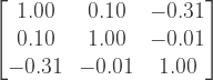
As you can see, each series exhibits autocorrelation, but the three series don’t really seem to move in the same directions. So then, I multiply all those random numbers in the graph with the Cholesky decomposition of the correlation matrix. Let’s say that this time we’ll go with higher correlations:

$\textbf{C} = \begin{bmatrix} 1.0 & 0.8 & 0.8 \\ 0.8 & 1.0 & 0.8 \\ 0.8 & 0.8 & 1.0\end{bmatrix}$

So that the Cholesky decomposition is:

$\textbf{L} = \begin{bmatrix} 1.0000 & 0.8000 & 0.8000 \\ 0.0000 & 0.6000 & 0.2667 \\ 0.0000 & 0.0000 & 0.5375\end{bmatrix}$

Again we just multiply the cross-sectionally uncorrelated (but autocorrelated!) series with the Cholesky decomposition to get the cross-correlated ánd autocorrelated series, as shown in the graph below:

And you’re done. The graph clearly shows both autocorrelaton within the series as cross-correlation between the series.

5. Conclusion

You now already know a lot about simulation. You know how to simulate random numbers between 0 and 1. You know that you can interpret those numbers as probabilities, such that you can translate them into values coming from any probability distribution, for example a normal distribution. You also know what cross-correlation and autocorrelation means, and how to introduce it in your simulations. Excel is pretty good for simulation. I always start in Excel, and move to MATLAB later on, because it’s much faster and has a lot more functions. I use simulation a lot in my job. I use it to simulate defaults of different companies, because those defaults impact bank losses. I use it to estimate the bias in some models. I use it to judge the performance of different statistical techniques, and so on. A long time ago, I used to do it to evaluate different poker strategies. You can do a lot of nice things. Just don’t forget your economic intuition, because you’ll need it, I’m sure.

VBA code for a Cholesky decomposition.

Just put this code in a module in Excel Developer and use the CHOL() function in Excel. Remember to first select the appropriate number of cells (i.e. the same dimensions as your correlation matrix). Then type ‘CHOL(‘, select your entire correlation matrix and then type ‘)’. Now press Ctrl+Shift+Enter to let Excel know you’re dealing with matrices. The Cholesky decomposition will pop up. Always make sure your correlation matrix is positive semi-definite! Also, in MATLAB you can simply calculate the Cholesky decomposition with the chol() function.

The code (most of it is stolen from this website)

Function CHOL(matrix As Range)

Dim i As Integer, j As Integer, k As Integer, N As Integer
Dim a() As Double 'the original matrix
Dim element As Double
Dim L_Lower() As Double

N = matrix.Columns.Count

ReDim a(1 To N, 1 To N)
ReDim L_Lower(1 To N, 1 To N)

For i = 1 To N
    For j = 1 To N
        a(i, j) = matrix(i, j).Value
        L_Lower(i, j) = 0
    Next j
Next i

For i = 1 To N
    For j = 1 To N
        element = a(i, j)
        For k = 1 To i - 1
            element = element - L_Lower(i, k) * L_Lower(j, k)
        Next k
        If i = j Then
            L_Lower(i, i) = Sqr(element)
        ElseIf i < j Then
            L_Lower(j, i) = element / L_Lower(i, i)
        End If
    Next j
Next i

CHOL = Application.WorksheetFunction.Transpose(L_Lower)

End Function

De blog van Kurt

Nothing disciplines and organises thinking as much as writing…

Simulation: simulating uncorrelated and correlated random variables

1. Simulating random numbers and uncorrelated random variables

2. Simulating correlated random variables (e.g. stock returns)

3. Simulating autocorrelated random variables (e.g. GDP growth)

4. Simulating random variables with autocorrelation AND cross-correlation

5. Conclusion

2 gedachten over “Simulation: simulating uncorrelated and correlated random variables”

Plaats een reactie Reactie annuleren

De blog van Kurt

Nothing disciplines and organises thinking as much as writing…

1. Simulating random numbers and uncorrelated random variables

2. Simulating correlated random variables (e.g. stock returns)

3. Simulating autocorrelated random variables (e.g. GDP growth)

4. Simulating random variables with autocorrelation AND cross-correlation

5. Conclusion

Dit delen:

Gerelateerd

2 gedachten over “Simulation: simulating uncorrelated and correlated random variables”

Plaats een reactie Reactie annuleren